


Step-by-Step Guide to Sizing a Crossover
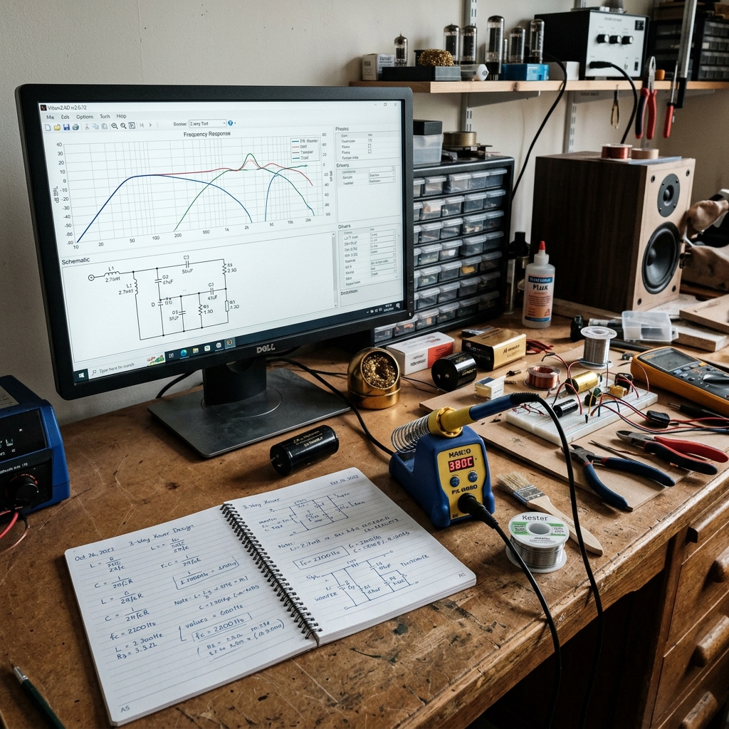
Once you understand speaker parameters and know what component quality is required for a good crossover, the next step is the actual sizing: what size capacitor do you need, what size inductor, and what filter topology should you choose? This article covers exactly that—from the formulas to the simulation workflow, while also addressing the most common mistakes that even experienced builders make.
The Basic Principles of Crossover Design
What is the crossover frequency, and how is it calculated?
The most important parameter of a crossover is the crossover frequency (fc)—the point at which the passband of one filter branch decreases in accordance with the chosen topology (typically −3 dB for a single first- or second-order section, and in the case of Linkwitz–Riley summing, the combined flat response of the two branches is often −6 dB per branch at the crossover point). This is not chosen arbitrarily: it is determined by the physical behavior of the loudspeaker, its upper and lower operating limits, and the bidirectional sound pressure summation.
General rules for determining fc:
- The upper operating limit of the subwoofer is not determined by Fs, but rather by diaphragm breakup (cone resonances) and directivity (beaming): Based on the measured frequency and off-axis response curves, the cutoff point should be set well below the first breakup peak and at a point where the subwoofer’s radiation angle still aligns with that of the tweeter.
- The lower limit of the tweeter is determined by the minimum operating frequency specified by the manufacturer (typically 1.5–3 kHz) and the measured frequency response at its maximum rated power.
- When determining the crossover range, the phase relationship must also be taken into account — the two filter branches must not reinforce or cancel each other out in the crossover band (unless you do so intentionally for dipole compensation or baffle step correction).
Why isn’t a calculator enough?
There are many online calculators that immediately spit out the inductor and capacitor values once you enter fc and impedance. These would be accurate in an ideal system—but in reality:
- The speaker’s impedance is frequency-dependent, not constant (8 Ω is not 8 Ω at every frequency)
- The speaker’s natural resonance peak on the impedance graph affects the filter’s behavior
- The DCR of the inductor acts as an additional series resistance, distorting the calculated crossover point
- The ESR of the capacitor also modifies the filter’s behavior
Therefore, the calculation provides a starting point, but measurement and simulation (using actual impedance data) yield the final result.
Basic Formulas — for 1st- and 2nd-order Filters
First-order filters
First-order low-pass (LPF) and high-pass (HPF) filters are the simplest—both consist of a single reactive element.
First-order low-pass (for subwoofers, series inductor):
L = Z / (2π × fc)where:
- L = inductance (in henries), then converted to mH
- Z = nominal impedance of the loudspeaker (Ω)
- fc = desired cutoff frequency (Hz)
Example: fc = 2000 Hz, Z = 8 Ω
L = 8 / (2π × 2000) = 8 / 12566 ≈ 0.000637 H = 0.637 mH
First-order high-pass filter (for a tweeter, series capacitor):
C = 1 / (2π × fc × Z)Example: fc = 2000 Hz, Z = 8 Ω
C = 1 / (2π × 2000 × 8) = 1 / 100531 ≈ 0.00000994 F = 9.94 µF
Second-order filters — Butterworth and Linkwitz–Riley
Second-order filters contain one of each type (L and C). The calculation depends on the desired filter characteristic (Butterworth vs. Linkwitz–Riley).
2nd-order Butterworth low-pass filter:
L = (Z × √2) / (2π × fc) C = 1 / (√2 × 2π × fc × Z)The factor √2 (≈ 1.414) follows from the Butterworth filter’s Q value of 0.707.
Example: fc = 2000 Hz, Z = 8 Ω
L = (8 × 1.414) / (2π × 2000) = 11.314 / 12566 ≈ 0.9 mH
C = 1 / (1.414 × 2π × 2000 × 8) = 1 / 142165 ≈ 7.03 µF
2nd-order Linkwitz–Riley (LR2) low-pass / high-pass filter (ideal R load, fc cutoff frequency):
The LR2 contains one LC pair per branch (not a single L or C, as in the first order). To ensure that the sum of the two branches remains flat, the section is tuned to second-order behavior with Q = 0.5—this is not the same as the value of a single first-order element.
Low-pass (series L, followed by a parallel C branch leading to the load Z and then to ground—the typical “L in series, C in shunt” topology in passive crossovers):
L = Z / (π × fc) = 2Z / (2π × fc) C = 1 / (4π × fc × Z) = 0.5 / (2π × fc × Z)Example: fc = 2000 Hz, Z = 8 Ω
L = 8 / (π × 2000) ≈ 1.27 mH
C = 1 / (4π × 2000 × 8) ≈ 4.97 µF
For comparison, in a first-order filter with the same parameters, L = Z/(2πfc) ≈ 0.637 mH, C = 1/(2πfcZ) ≈ 9.94 µF — thus, the LR2 requires twice the L and half the C of the first-order section (it also has a larger L and smaller C compared to the Butterworth filter: Q = 0.5 instead of 0.707).
The high-pass branch can be calculated symmetrically (C in series, L in shunt) from this same duality: C = 1/(4π fc Z), L = Z/(π fc) (the same structure, with L and C swapped in the corresponding topology).
In a real passive network, the exact values are shifted due to the coil’s DCR, the capacitor’s ESR, and the speaker’s Z(f) curve—the above formulas provide an initial estimate; the final values require VituixCAD (or another pole-based simulator) and measurement.
4th-order Linkwitz–Riley (LR4)—the professional standard
The LR4 consists of a cascade of two second-order Butterworth sections at the same fc (total slope of 24 dB/octave, typically −6 dB per branch at the cutoff point for electrical summation). Passive L–C–L–C ladder (series L, shunt C, series L, shunt C, followed by the Z load), the approximate component formulas derived from synthesis—often cited in DIY contexts—are as follows (fc in Hz, Z in Ω, result in henries/farads):
L1 = 0.30 × Z / fc C1 = 0.2533 / (Z × fc) L2 = 0.15 × Z / fc C2 = 0.0563 / (Z × fc)Example: fc = 2000 Hz, Z = 8 Ω
L1 ≈ 1.20 mH, C1 ≈ 15.8 µF, L2 ≈ 0.60 mH, C2 ≈ 3.52 µF
These factors apply to this specific passive ladder topology; for other configurations (e.g., different order, center tap, or HPF symmetry in the high-pass branch), the values must be recalculated. Instead of manual calculations, in practice, the simulator’s built-in LR4/Butterworth wizard offers the least potential for error—the above sequence serves as a verifiable starting point for the 8 Ω / 2 kHz range.
Impedance Compensation — the Zobel Network
The inductance (Le) of the speaker causes a rise in the impedance curve at high frequencies. For example, a speaker with a nominal impedance of 8 Ω may exhibit an impedance of 15–25 Ω at 10 kHz. This shifts the actual cutoff frequency of the high-pass filter.
A Zobel network is a series RC combination connected in parallel with the speaker. Its purpose is to compensate for the rise in impedance caused by inductance.
Zobel calculation:
R_zobel = Re × 1.25 (rule of thumb: between Re × 1.0 and 1.5) C_zobel = Le / Re² (approximation — refine by measurement)where Re is the DC resistance of the speaker, and Le is its inductance (in H). The relationship C_zobel = Le/Re² is a simplified estimate: in practice, the frequency-dependent impedance of the voice coil and motor should be adjusted based on the complex equation and the measured Z(f) curve — the goal is for the impedance to be as flat as possible in the frequency band relevant to the filter after the Zobel network is installed.
Example: Re = 6 Ω, Le = 0.5 mH = 0.0005 H
R_zobel = 6 × 1.25 = 7.5 Ω (nearest standard: 7.5 Ω)
C_Zobel = 0.0005 / 36 = 0.0000139 F = 13.9 µF (nearest standard: 15 µF)
It is advisable to fine-tune the actual values based on measurement results: the impedance curve should be flat across the entire frequency range after the Zobel network is installed.
Compensating for the resonance peak — “notch” / trap filter
The speaker’s impedance peak around Fs can also affect the low-pass filter’s behavior, especially if the crossover point is close to Fs. A common solution is a branch connected in parallel with the speaker, which provides a higher load around Fs (to “suck out” the resonance)—also referred to as a trap or notch in DIY articles.
The most straightforward starting model: an L and C connected in series in parallel with the speaker, tuned so that the series resonance frequency is Fs:
ω₀ = 2π × Fs Choose a C value (standard series), then: L = 1 / (ω₀² × C) (ekkor ω₀² = 1/(L×C) )The role of R (resistance): it fine-tunes the resonance Q / bandwidth and the fit of the measured impedance curve—in a passive network, this is not a single “universal” formula, but rather the result of simulation (Z(f) + trap) and impedance measurement. The Thiele–Small Qms / Qes parameters are part of the mechanical–electrical model; it is not practical to “compress” the specific trap components directly into a single formula—the reliable approach is measurement-driven fine-tuning.
If Fs is far from the breakpoint and the filter’s slope already suppresses the peak, a good result is possible even without a trap—the simulated and measured impedances always determine the outcome.
L-pad Level Equalization
In a two-way speaker system, the efficiency of the woofer and tweeter usually differs. If the tweeter is 3 dB louder, this must be compensated for—otherwise, the frequency response will show a dip in the crossover band.
The L-pad consists of two resistors: one in series (Rs) and one in parallel with the driver (Rp), which together provide attenuation so that the apparent impedance remains close to the nominal Z.
Role in the diagram: Rs is in the signal path before the driver (moving from the amplifier toward the tweeter: first Rs, then the junction); Rp is a shunt connected between the driver’s two terminals (in parallel with the speaker itself). This allows the formula to be clearly matched to the component placement.
L-pad calculation for a given dB attenuation and impedance:
If the desired attenuation in dB is A, and the nominal impedance is Z,
Attenuation ratio: r = 10^(A/20) Rs = Z × (r - 1) / r Rp = Z / (r - 1)Example:
3 dB attenuation, Z = 8 Ω
r = 10^(3/20) = 10^0.15 ≈ 1.413
Rs = 8 × (1.413 - 1) / 1.413 = 8 × 0.292 = 2.33 Ω
(nearest standard: 2.2 Ω)
Rp = 8 / 0.413 = 19.4 Ω
(nearest standard: 20 Ω)
The finished L-pad fits between the high-frequency driver’s filter and the tweeter (Rs in series, Rp in parallel with the tweeter). The exact topology of the passive HPF (where the series C is located relative to Rs) can affect the apparent reactance—always simulate the entire branch; do not just calculate the resistors in isolation.
Simulation Workflow with VituixCAD
VituixCAD (free, Windows) remains the best free software available today for full speaker simulation. The process:
1. Importing measured data
Load the impedance and frequency response data (.txt or .frd format) measured with REW for each individual speaker. Based on this data, VituixCAD simulates how the entire system will sound.
Important: Measurements should be taken across the entire speaker baffle (including baffle step compensation) whenever possible, not in free space. The size of the baffle (front panel) affects diffraction behavior, and the simulator needs to account for this.
2. Setting Crossover Values
In the VituixCAD graphical interface, you specify the filter topology (1st, 2nd, 3rd, or 4th order, LPF/HPF) and the component values. The simulator immediately displays:
- The frequency response of each branch
- The combined frequency response (sum)
- The phase response
- The group delay
- The impedance plot for the entire system
3. Optimization
VituixCAD includes a built-in optimizer: you specify a target characteristic (e.g., Harman curve approximation or a flat ±1 dB response between 200 and 15,000 Hz), and the optimizer automatically finds the best component values. The optimizer’s result isn’t always practical (e.g., it might recommend a 7.32 µF capacitor, which can be achieved by combining standard components), but it provides a good starting point.
4. Baffle Step Compensation
Due to the speaker’s front panel (baffle), low frequencies radiate into the entire space (4π), while higher frequencies radiate only forward into the half-space (2π): the speaker’s on-axis level thus rises by approximately 6 dB relative to the low-frequency range in a transition band centered around 200–800 Hz, depending on the width of the front panel. Without compensation, the sound image will be thin and lack bass. The VituixCAD baffle step simulator shows the expected deviation, which can be automatically taken into account when designing the crossover.
Practical Component Value Rounding and Combining
Calculations rarely yield exact standard component values (e.g., 6.38 µF or 0.73 mH). The solution: available values can be combined using parallel or series connections.
Parallel connection of capacitors:
C_total = C1 + C2
For example: 5.6 µF + 1.5 µF = 7.1 µF (an approximation instead of 6.8 µF)
Series connection of inductors:
L_total = L1 + L2
For example: 0.68 mH + 0.10 mH = 0.78 mH
For resistors: Series = sum; parallel = reciprocal of the sum.
Premium capacitor manufacturers (e.g., Mundorf, Jantzen) offer a narrower range of values, but these values have finer increments and tighter tolerances (±1–2%). This means fewer combinations are needed to achieve the ideal values.
The most common mistakes in crossover design
1. Calculations are based on nominal impedance, not measured impedance
An 8 Ω nominal speaker can easily exhibit an impedance of 10–14 Ω at the crossover frequency. If you do not take this into account when calculating fc, the actual crossover frequency may differ by 10–20% from the designed value.
Solution: Plot the impedance curve (using DATS v3 or REW) and calculate using the actual impedance value around fc—or simulate using real impedance data.
2. DCR is ignored
If the coil’s DCR is, for example, 0.8 Ω, and the speaker’s Re is 6 Ω, then the actual resistance of the coil plus the speaker is 6.8 Ω—not 6 Ω. This affects both the Q-factor and the effective breakpoint.
Solution: Add the DCR to Re in the calculation. In simulations, VituixCAD allows you to adjust the component’s DCR.
3. They don’t measure—they just simulate
A simulation is only as good as its input data. Rely on your own measurements rather than manufacturer data sheets—especially if the speaker isn’t new or if it’s operating in a specific enclosure or baffle.
4. Phase relationships are not checked
In the crossover region, the phases of the individual filter branches do not automatically match. If there is a 180° phase difference, the speakers will cancel each other out in the crossover band—this causes a deep “dip” in the frequency response. The solution: reverse the polarity of the tweeter (or choose a different filter topology).
5. They aren’t tested under real-world listening conditions
A crossover that performs perfectly in a simulation can sound terrible when listened to in a poorly designed room—but the reverse is also true: a crossover that isn’t ideal in a simulation can perform well under real-world conditions. The final test is always listening and measurement under the actual placement conditions.
A step-by-step example of designing a specific 2-way speaker
Initial data:
- Subwoofer: SB Acoustics, nominal impedance 8 Ω, measured impedance at 2000 Hz: 12 Ω, Le ≈ 0.6 mH, Re = 6.2 Ω
- Tweeter: SB Acoustics dome tweeter, nominal impedance 8 Ω, measured impedance at 2000 Hz: 9 Ω
- Desired fc = 2000 Hz, topology: 2nd-order Butterworth (approximation, refined via simulation)
Woofer LPF (2nd-order Butterworth, Z = 12 Ω at fc):
L = (12 × √2) / (2π × 2000) = 16.97 / 12,566 ≈ 1.35 mH
C = 1 / (1.414 × 2π × 2000 × 12) = 1 / 213,255 ≈ 4.7 µF
Rounding: L = 1.2 mH + 0.15 mH (in series) = 1.35 mH; C = 4.7 µF (standard value) ✓
Zobel network for the subwoofer (Le = 0.6 mH, Re = 6.2 Ω):
R_zobel = 6.2 × 1.25 = 7.75 Ω → standard: 7.5 Ω
C_Zobel = 0.0006 / (6.2²) = 0.0006 / 38.44 ≈ 15.6 µF → standard: 15 µF
Tweeter HPF (2nd-order Butterworth, Z = 9 Ω at fc):
C = 1 / (1.414 × 2π × 2000 × 9) = 1 / 159936 ≈ 6.25 µF
L = (9 × √2) / (2π × 2000) = 12.73 / 12566 ≈ 1.01 mH
Rounding: C = 5.6 µF + 0.68 µF = 6.28 µF (final correction via simulation); L = 1.0 mH ✓
Level balancing:
If the tweeter is 2 dB louder (based on measurements):
r = 10^(2/20) ≈ 1.259
Rs = 9 × 0.259 / 1.259 ≈ 1.85 Ω
→ standard: 1.8 Ω
Rp = 9 / 0.259 ≈ 34.7 Ω
→ standard: 33 Ω
This is the starting point. Once the measured speaker data is loaded into VituixCAD and using these values as a baseline, the optimizer fine-tunes the values—and the result is a measurably flat, phase-coherent crossover.
Summary
Crossover design isn’t black magic—but it’s not just about using a calculator either. The process:
- Start with measured data—not the manufacturer’s spec sheet.
- Calculate using formulas based on fc and Z, taking actual impedance values into account.
- Compensate for inductance with a Zobel network, and if necessary, use a notch filter to counteract the resonance peak.
- Simulate with VituixCAD using actual measured data—and check the phase relationship.
- Measure every component with an LCR meter and select matching pairs.
- Iterate—measure the frequency response on the finished speaker, then fine-tune.
If you go through this entire process, the result will not only meet your own expectations—it will be a reproducible speaker backed by objective measurement data. This is the point where DIY speaker building ceases to be a hobby and becomes an engineering endeavor.